This study material has been compiled from a lecture audio transcript and copy-pasted text (likely from slides or a textbook).
📚 Risk and Uncertainty: A Comprehensive Study Guide
🎯 Introduction to Decision-Making Under Risk and Uncertainty
Decision theory often distinguishes between situations involving risk and those involving uncertainty. Understanding this fundamental difference is crucial for analyzing how individuals and organizations make choices when outcomes are not guaranteed.
1️⃣ Risk vs. Uncertainty
- Risk 🎲: Refers to situations where the probabilities of various outcomes are known or can be objectively determined.
- Example: Tossing a fair coin, where the probability of heads or tails is 1/2.
- Representation: A lottery (L), defined as a set of outcomes (x) each associated with a known probability (p).
L = (p1: x1, p2: x2, ..., pn: xn)- This means outcome
x1occurs with probabilityp1,x2withp2, and so on.
- Uncertainty ❓: Describes situations where the probabilities of outcomes are unknown or cannot be objectively determined.
- Example: Predicting the success of a new product launch, where many factors have unknown probabilities.
- Representation: An act (A), where outcomes (x) are associated with states of the world (s) rather than known probabilities.
A = (s1: x1, s2: x2, ..., sn: xn)- If state
s1occurs, outcomex1results, and so forth.
2️⃣ Choice Under Risk: Expected Utility Theory
Expected Utility Theory (EUT) is a cornerstone of standard economics for understanding how individuals make choices when facing risky outcomes.
2.1 Expected Value (EV) vs. Expected Utility (EU)
- Expected Value (EV) 📈: The average outcome expected if a lottery were played many times.
- Formula:
EV(L) = p1x1 + p2x2 + ... + pnxn = Σ(pi * xi) - Limitation: EV often fails to capture how people actually make decisions, especially with large sums, as it doesn't account for subjective valuation.
- Formula:
- Expected Utility (EU) 🧠: Accounts for an individual's subjective valuation of outcomes.
- Formula:
EU(L) = p1u(x1) + p2u(x2) + ... + pnu(xn) = Σ(pi * u(xi)) u(x)is the utility function, which assigns a subjective value to each outcomex.- Key Remark: The utility function
uin EUT is cardinal, meaning differences in utility values are meaningful, not just their order.
- Formula:
2.2 The St. Petersburg Paradox 🤯
This paradox highlights the limitations of EV and the necessity of EU.
- Game: A fair coin is tossed repeatedly until heads appears. If it takes
ntosses, you win2^neuros. - Expected Value:
EV = (1/2)*2 + (1/4)*4 + (1/8)*8 + ... = 1 + 1 + 1 + ... = ∞ - Paradox: Despite an infinite EV, most people are only willing to pay a small amount to play.
- Resolution with EU: If we assume a logarithmic utility function, e.g.,
u(x) = ln(x), the EU becomes finite (EU ≈ 1.39), aligning better with observed behavior. This suggests people value additional wealth less as their total wealth increases.
2.3 Risk Attitudes
An individual's attitude towards risk is reflected in their preferences and the shape of their utility function.
- Risk-Averse 📉: Prefers the Expected Value of a lottery for sure over the lottery itself.
(100%: EV(L)) ≻ L- Certainty Equivalent (CE):
CE(L) < EV(L)(willing to accept a lower sure amount to avoid risk). - Utility Function Shape: Concave (marginal utility of wealth decreases as wealth increases).
- Risk-Neutral ⚖️: Indifferent between the Expected Value for sure and the lottery.
(100%: EV(L)) ~ L- Certainty Equivalent (CE):
CE(L) = EV(L). - Utility Function Shape: Linear (constant marginal utility).
- Risk-Seeking 📈: Prefers the lottery over its Expected Value for sure.
(100%: EV(L)) ≺ L- Certainty Equivalent (CE):
CE(L) > EV(L)(requires a higher sure amount to forgo the potential upside). - Utility Function Shape: Convex (marginal utility of wealth increases with wealth).
3️⃣ Violations of Expected Utility Under Risk
While EUT is a powerful normative model (how people should decide), it often fails descriptively (how people actually decide).
3.1 The Asian Disease Problem 🏥
This problem demonstrates how framing affects decision-making, violating EUT.
- Scenario: US prepares for an outbreak expected to kill 600 people.
- Frame 1 (Gains):
- Program A: Saves 200 people (for sure).
- Program B: 1/3 probability of saving 600 people, 2/3 probability of saving 0.
- Typical Choice: Most favor Program A (risk-averse for gains).
- Frame 2 (Losses):
- Program C: 400 people die (for sure).
- Program D: 1/3 probability of 0 people dying, 2/3 probability of 600 people dying.
- Typical Choice: Most favor Program D (risk-seeking for losses).
- Frame 1 (Gains):
- Violation: The two scenarios are objectively identical (e.g., saving 200 is equivalent to 400 dying out of 600), yet preferences reverse due to framing.
- Consistency with Prospect Theory:
- Reference Points: Outcomes are evaluated as gains or losses relative to a baseline (e.g., 'nobody saved' or 'nobody dies').
- Diminishing Sensitivity: A change from 0 to 10 feels larger than 100 to 110, for both gains and losses. This implies utility is concave for gains and convex for losses.
- Reflection Effect: Risk attitudes for gains are opposite to those for losses (risk-averse for gains, risk-seeking for losses).
- Loss Aversion: Losses loom larger than equivalent gains. The utility function is steeper for losses than for gains around the origin (
|u(-x)| > |u(+x)|for smallx > 0).
3.2 The Allais Paradox 🎰
This paradox demonstrates a violation of the Sure Thing Principle, a core axiom of EUT.
- Sure Thing Principle: If two alternatives share a common outcome in a specific state, the preference between them should not depend on that common outcome.
- Choices:
- Choice 1:
- A: (0.10: €5M, 0.89: €1M, 0.01: €0)
- B: (1.00: €1M)
- Typical Choice: Most prefer B (certainty of €1M). So,
A ≺ B.
- Choice 2:
- C: (0.10: €5M, 0.90: €0)
- D: (0.11: €1M, 0.89: €0)
- Typical Choice: Most prefer C (higher potential gain, even with higher risk). So,
C ≻ D.
- Choice 1:
- Violation: These preferences (
A ≺ BandC ≻ D) are inconsistent with EUT. IfA ≺ B, then0.10 u(5M) + 0.01 u(0) < 0.11 u(1M). This inequality, when0.89 u(0)is added to both sides, impliesC ≺ D, which contradicts the observed preferenceC ≻ D. - Consistency with Certainty Effect: People tend to overweight outcomes that are certain, leading to a strong preference for the sure €1M in Choice 1.
4️⃣ Choice Under Uncertainty: Simple Models
When probabilities are unknown, EUT cannot be directly applied without subjective probabilities. Simpler decision rules are sometimes used.
- Maximin ✅: Choose the alternative with the greatest minimum utility payoff. (Pessimistic approach)
- Example: If "Rain" leads to "Wet, miserable" (low utility) and "No Rain" leads to "Dry, not happy" (medium utility), Maximin would choose the option that maximizes the worst-case outcome.
- Maximax ✅: Choose the alternative with the greatest maximum utility payoff. (Optimistic approach)
- Example: If "Rain" leads to "Wet, miserable" and "No Rain" leads to "Dry, happy" (high utility), Maximax would choose the option that maximizes the best-case outcome.
- Minimax-Regret ✅: Choose the alternative with the lowest maximum regret. Regret is the difference between the best possible outcome for a given state and the outcome of the chosen alternative for that state.
- Example: If choosing "Dry, not happy" when it rains leads to a regret of 3 (because "Wet, miserable" would have been 0 regret), and choosing "Wet, miserable" when it doesn't rain leads to a regret of 5, Minimax-regret aims to minimize the largest potential regret.
- Limitation: These models do not account for beliefs about the likelihoods of states.
- Subjective Expected Utility (SEU) 💡: A more advanced approach where subjective probabilities are assigned to all states of the world, and then EUT is applied.
5️⃣ Violations of Expected Utility Under Uncertainty
5.1 The Ellsberg Paradox 🏺
This paradox demonstrates ambiguity aversion, a preference for known risks over unknown risks, violating SEU.
- Setup: An urn contains 90 balls: 30 are red (R), and 60 are either black (B) or yellow (Y) in unknown proportions.
- Choices:
- Bet 1:
- I: Bet on Red (Win €100 if R, €0 otherwise)
- II: Bet on Black (Win €100 if B, €0 otherwise)
- Typical Choice: Most prefer I over II (
I ≻ II), as the probability of Red (1/3) is known, while Black's probability is ambiguous.
- Bet 2:
- III: Bet on Red or Yellow (Win €100 if R or Y, €0 otherwise)
- IV: Bet on Black or Yellow (Win €100 if B or Y, €0 otherwise)
- Typical Choice: Most prefer IV over III (
IV ≻ III), as the probability of (Black or Yellow) is known (2/3), while (Red or Yellow)'s probability is ambiguous.
- Bet 1:
- Violation: These preferences are inconsistent with SEU.
I ≻ IIimpliesP(R) > P(B).IV ≻ IIIimpliesP(B) + P(Y) > P(R) + P(Y), which simplifies toP(B) > P(R).- These two implications contradict each other.
- Consistency with Ambiguity Aversion: People prefer situations where probabilities are known (Bet I and IV) over those where probabilities are ambiguous (Bet II and III).